Per-unit tax graph: tax incidence, tax revenue and deadweight loss

An example figure from the Supply and Demand generator.

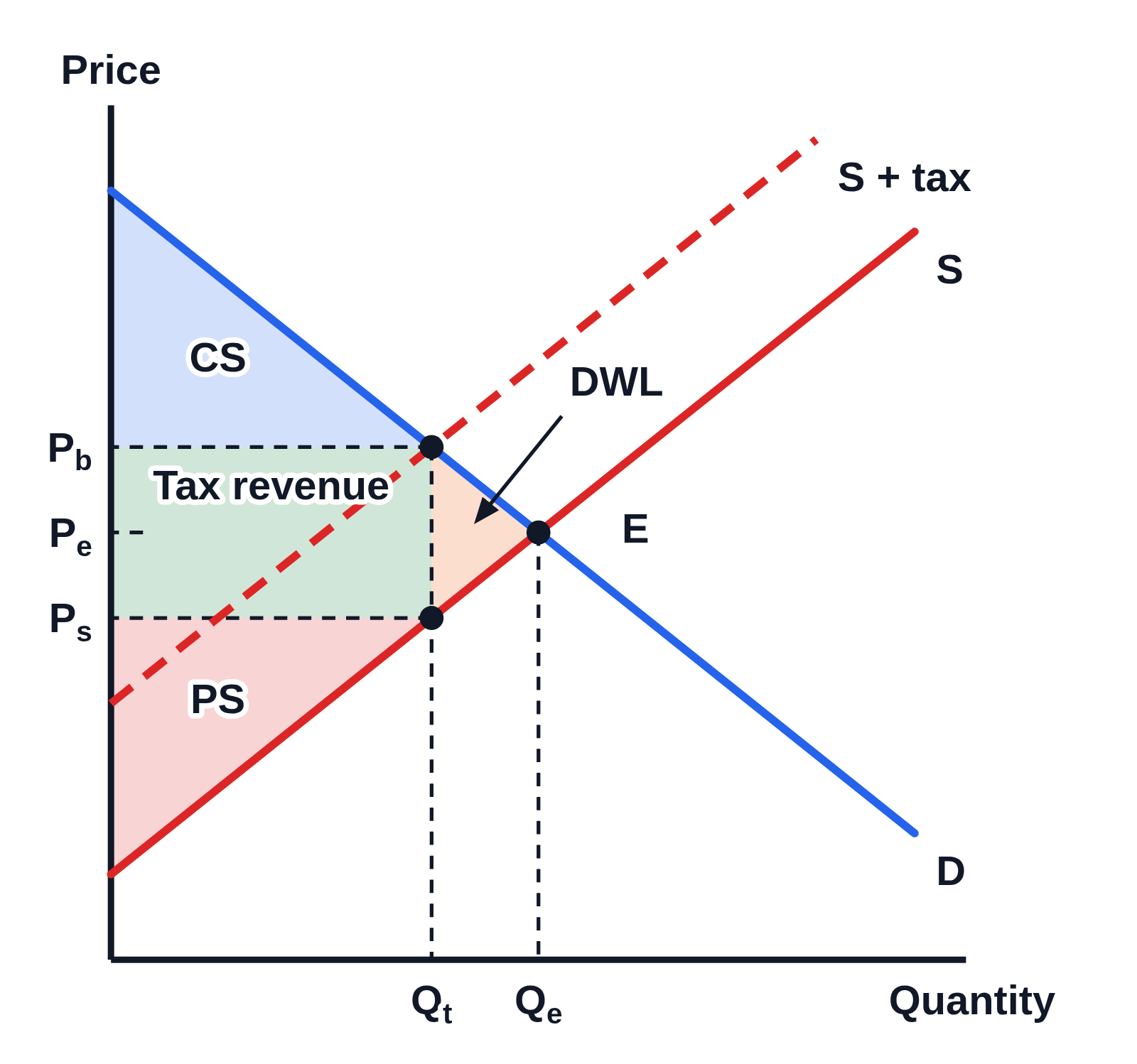
Supply and demand graph with no numbers on the axes, Price up the side and Quantity along the bottom: demand D and supply S crossing at E, and a dashed curve S + tax above S. Dashed lines mark Pb and Ps on the price axis, above and below Pₑ, the height of E, which has only a short dash at the axis, and Qt left of Qₑ on the quantity axis. Shaded regions are labeled CS in blue above Pb, Tax revenue in green between Ps and Pb out to Qt, PS in red below Ps, and DWL in orange, written above and right of the small triangle between Qt and Qₑ with an arrow to it — A per-unit tax shifts the supply curve up from S to the dashed S + tax. Buyers now pay Pb, more than the price at the old equilibrium E, sellers keep Ps, less than it, and the quantity sold falls from Qₑ to Qt. The shaded areas show consumer surplus (CS), producer surplus (PS), the tax revenue between Ps and Pb, and the deadweight loss (DWL) between Qt and Qₑ.

Edit this figure Download PNG

Editing opens it in Supply and Demand with these settings, to change anything and copy or download your own.

Free to use in your tests, worksheets, slides or anything else, no credit needed. Public domain under CC0 1.0. How to reuse our figures

More Supply and Demand examples

Make your own in Supply and Demand →